In-class_Ex06

Installing and Loading the R packages

Before we get started, we need to ensure that sfdep, sf, tmap and tidyverse packages of R are currently installed in your R.

pacman::p_load(sf, sfdep, tmap, tidyverse)

The Data

For the purpose of this in-class exercise, the hunan data sets will be used. There are two data sets in this use case, they are:

• Hunan, a goaspatial data set in ESRI shapefile format, and
• Hunan_2021, an attribute data set in csv format.

Importing geospatial data

hunan <- st_read(dsn = "data/Geospatial", 
                 layer = "Hunan")

Reading layer `Hunan' from data source 
  `C:\Users\kwekm\Desktop\SMU Year 3 Semester 2\IS415 Geospatial Analytics and Applications\KMRCrazyDuck\IS415-KMR\In-class_Ex\Data\Geospatial' 
  using driver `ESRI Shapefile'
Simple feature collection with 88 features and 7 fields
Geometry type: POLYGON
Dimension:     XY
Bounding box:  xmin: 108.7831 ymin: 24.6342 xmax: 114.2544 ymax: 30.12812
Geodetic CRS:  WGS 84

Import csv file into r environment

hunan2012 <- read_csv("data/Aspatial/Hunan_2012.csv")

Performing relational join

The code chunk below will be used to update the attribute table of hunan’s SpatialPolygonsDataFrame with the attribute fields of hunan2012 dataframe. This is performed by using left_join() of dplyr package.

hunan_GDPPC <- left_join(hunan,hunan2012)%>%
  select(1:4, 7, 15)

tmap_mode("plot")
tm_shape(hunan_GDPPC) +
  tm_fill("GDPPC",
          style = "quantile",
          palette = "Blues",
          title = "GDPPC") +
    tm_layout(main.title = 'Distribution of GDP per capita by distribution',
    main.title.position = "center",
    main.title.size = 1.2,
    legend.height = 0.45,
    legend.width = 0.35,
    frame = TRUE) +
tm_borders(alpha = 0.5) +
tm_compass(type="8star", size = 2) +
tm_scale_bar() +
tm_grid(alpha =0.2)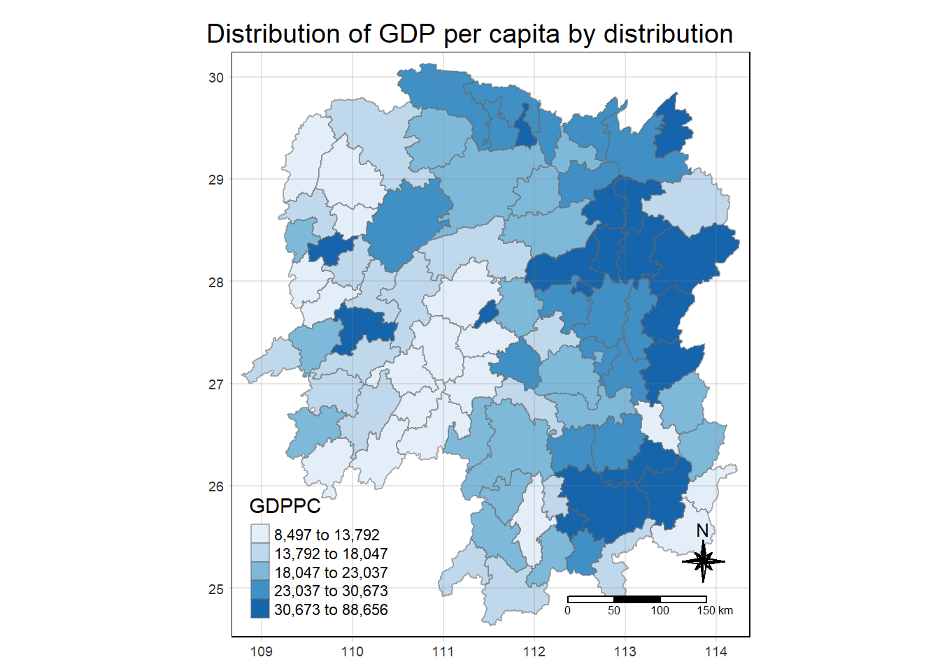

Visualising Regional Development Indicator

Now, we are going to prepare a basemap and a choropleth map showing the distribution of GDPPC 2012 by using qtm() of tmap package.

basemap <- tm_shape(hunan_GDPPC) +
  tm_polygons() +
  tm_text("NAME_3", size=0.5)

gdppc <- qtm(hunan_GDPPC, "GDPPC")
tmap_arrange(basemap, gdppc, asp=1, ncol=2)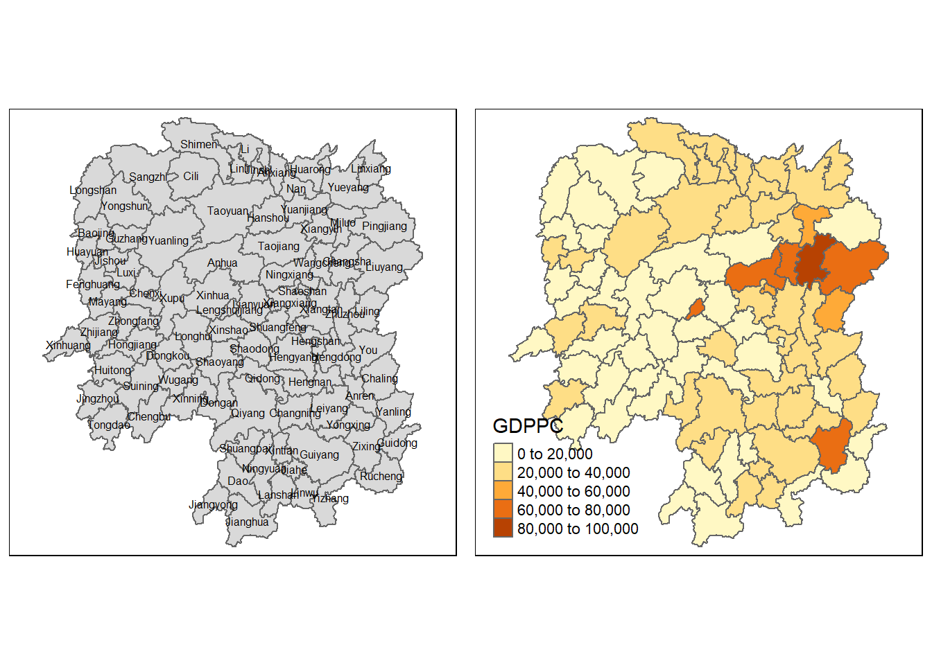

Contingency neighbours method

In the code chunk below, st_contiguity() is used to derive a continguity neighbour list by using queen’s method.

cn_queen <-hunan_GDPPC %>%
  mutate(nb = st_contiguity(geometry),
         .before = 1)

derive a contiguity neighbour list Using Rook’s method

cn_rook <- hunan_GDPPC %>%
  mutate(nb =st_contiguity(geometry),
         queen =FALSE,
         .before = 1)