In-class Exercise 7

Author

Kwek Ming Rong

Published

February 20, 2023

Modified

March 6, 2023

Global and Local Measures of Spatial Autocorrelation - SFDEP

Overview

In this hands-on exercise, you will learn how to compute Global and Local Measure of Spatial Autocorrelation (GLSA) by using spdep package. By the end to this hands-on exercise, you will be able to:

import geospatial data using appropriate function(s) of sf package,
import csv file using appropriate function of readr package,
perform relational join using appropriate join function of dplyr package,
compute Global Spatial Autocorrelation (GSA) statistics by using appropriate functions of spdep package,
- plot Moran scatterplot,
- compute and plot spatial correlogram using appropriate function of spdep package.
compute Local Indicator of Spatial Association (LISA) statistics for detecting clusters and outliers by using appropriate functions spdep package;
compute Getis-Ord’s Gi-statistics for detecting hot spot or/and cold spot area by using appropriate functions of spdep package; and
to visualise the analysis output by using tmap package.

1. Installing and Loading R packages

pacman::p_load(sf, sfdep, tmap, tidyverse, plotly, zoo, Kendall)

1.1 Importing the Geospatial Data

The code chunk below uses st_read() of sf package to import Hunan shapefile into R. The imported shapefile will be simple features Object of sf.

hunan <- st_read(dsn = "Data/Geospatial", 
                 layer = "Hunan")

Reading layer `Hunan' from data source 
  `C:\Users\kwekm\Desktop\SMU Year 3 Semester 2\IS415 Geospatial Analytics and Applications\KMRCrazyDuck\IS415-KMR\In-class_Ex\Data\Geospatial' 
  using driver `ESRI Shapefile'
Simple feature collection with 88 features and 7 fields
Geometry type: POLYGON
Dimension:     XY
Bounding box:  xmin: 108.7831 ymin: 24.6342 xmax: 114.2544 ymax: 30.12812
Geodetic CRS:  WGS 84

1.2 Importing CSV file into environment

Next, we will import Hunan_2012.csv into R by using read_csv() of readr package. The output is R dataframe class.

hunan2012 <- read_csv("Data/Aspatial/Hunan_2012.csv")

1.3 Performing relational join

The code chunk below will be used to update the attribute table of hunan’s SpatialPolygonsDataFrame with the attribute fields of hunan2012 dataframe. This is performed by using left_join() of dplyr package.

In order to retain the geospatial properties, the left data frame must be the sf data.frame (i.e. hunan)

hunan_GDPPC <- left_join(hunan,hunan2012)%>%
  select(1:4, 7, 15)

2. Plotting a Choropleth Map

tmap_mode("plot")
tm_shape(hunan_GDPPC) +
  tm_fill("GDPPC",
          style = "quantile", 
          palette = "Blues",
          title = "GDPPC") +
  tm_layout(main.title = "Distribution of GDP per captial by district",
            main.title.position = "center",
            main.title.size = 1.2,
            legend.height = 0.45,
            legend.width = 0.35,
            frame = TRUE) +
  tm_borders(alpha = 0.5) +
  tm_compass(type="8star", size = 2) +
  tm_scale_bar() + 
  tm_grid(alpha = 0.2)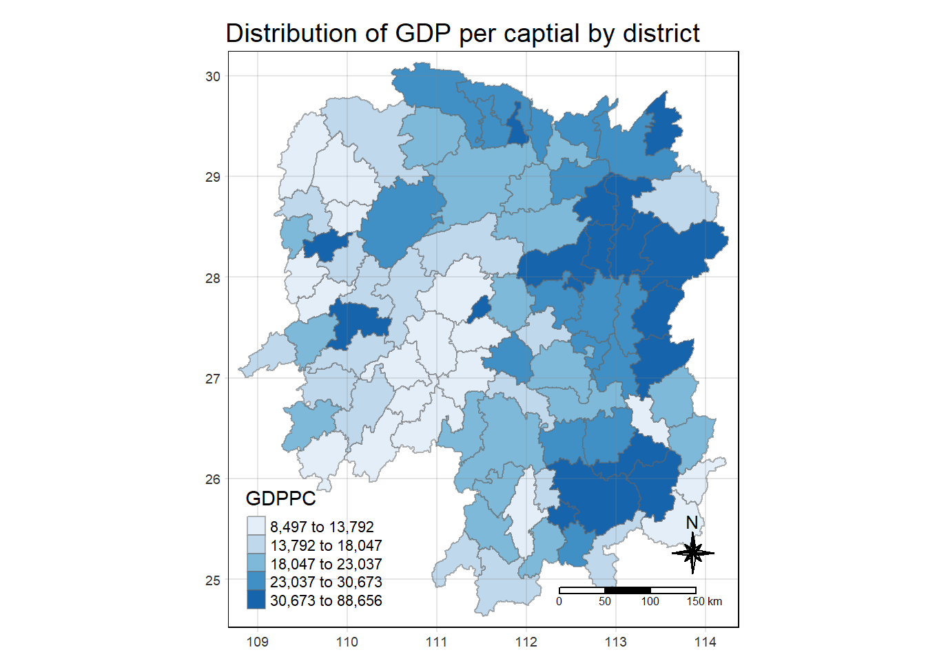

3. Deriving the contiguity weights

3.1 Contiguity weights: Queen’s method

wm_q <- hunan_GDPPC %>%
  mutate(nb = st_contiguity(geometry),
         wt = st_weights(nb,
                         style = "W"),
         .before = 1)

3.2 Contiguity weights: Rook’s method

wm_r <- hunan_GDPPC %>%
  mutate(nb = st_contiguity(geometry),
  queen = FALSE,
  wt = st_weights(nb,
                  style = "W"),
  .before = 1)

3.3 Computing Global Moran I

moranI <- global_moran(wm_q$GDPPC,
                        wm_q$nb,
                        wm_q$wt)

3.4 Performing Global Moran I’s Test

global_moran_test(wm_q$GDPPC,
                  wm_q$nb,
                  wm_q$wt)


    Moran I test under randomisation

data:  x  
weights: listw    

Moran I statistic standard deviate = 4.7351, p-value = 1.095e-06
alternative hypothesis: greater
sample estimates:
Moran I statistic       Expectation          Variance 
      0.300749970      -0.011494253       0.004348351

3.5 Performing Global Moran’s I permutation test

To ensure results stay the same when rendering every time

set.seed(1234)

global_moran_perm(wm_q$GDPPC,
                  wm_q$nb,
                  wm_q$wt,
                  nsim = 99)


    Monte-Carlo simulation of Moran I

data:  x 
weights: listw  
number of simulations + 1: 100 

statistic = 0.30075, observed rank = 100, p-value < 2.2e-16
alternative hypothesis: two.sided

If observation values are small, it is better to use a higher number of simulations

3.6 Computing local Moran’s I

lisa <- wm_q %>%
  mutate(local_moran = local_moran(
    GDPPC, nb, wt, nsim = 99),
    .before = 1) %>%
  unnest(local_moran)

lisa

Simple feature collection with 88 features and 20 fields
Geometry type: POLYGON
Dimension:     XY
Bounding box:  xmin: 108.7831 ymin: 24.6342 xmax: 114.2544 ymax: 30.12812
Geodetic CRS:  WGS 84
# A tibble: 88 × 21
         ii        eii   var_ii    z_ii    p_ii p_ii_…¹ p_fol…² skewn…³ kurtosis
      <dbl>      <dbl>    <dbl>   <dbl>   <dbl>   <dbl>   <dbl>   <dbl>    <dbl>
 1 -0.00147  0.00177    4.18e-4 -0.158  0.874      0.82    0.41  -0.812  0.652  
 2  0.0259   0.00641    1.05e-2  0.190  0.849      0.96    0.48  -1.09   1.89   
 3 -0.0120  -0.0374     1.02e-1  0.0796 0.937      0.76    0.38   0.824  0.0461 
 4  0.00102 -0.0000349  4.37e-6  0.506  0.613      0.64    0.32   1.04   1.61   
 5  0.0148  -0.00340    1.65e-3  0.449  0.654      0.5     0.25   1.64   3.96   
 6 -0.0388  -0.00339    5.45e-3 -0.480  0.631      0.82    0.41   0.614 -0.264  
 7  3.37    -0.198      1.41e+0  3.00   0.00266    0.08    0.04   1.46   2.74   
 8  1.56    -0.265      8.04e-1  2.04   0.0417     0.08    0.04   0.459 -0.519  
 9  4.42     0.0450     1.79e+0  3.27   0.00108    0.02    0.01   0.746 -0.00582
10 -0.399   -0.0505     8.59e-2 -1.19   0.234      0.28    0.14  -0.685  0.134  
# … with 78 more rows, 12 more variables: mean <fct>, median <fct>,
#   pysal <fct>, nb <nb>, wt <list>, NAME_2 <chr>, ID_3 <int>, NAME_3 <chr>,
#   ENGTYPE_3 <chr>, County <chr>, GDPPC <dbl>, geometry <POLYGON [°]>, and
#   abbreviated variable names ¹p_ii_sim, ²p_folded_sim, ³skewness

Variable mean and pysal value should be the same. For take home exercise 2, stay with mean

3.7 Visualising local Moran’s I

3.7.1 Computing ii

tmap_mode("plot")
tm_shape(lisa) +
  tm_fill("ii") +
  tm_borders(alpha = 0.5) +
  tm_view(set.zoom.limits = c(6,8))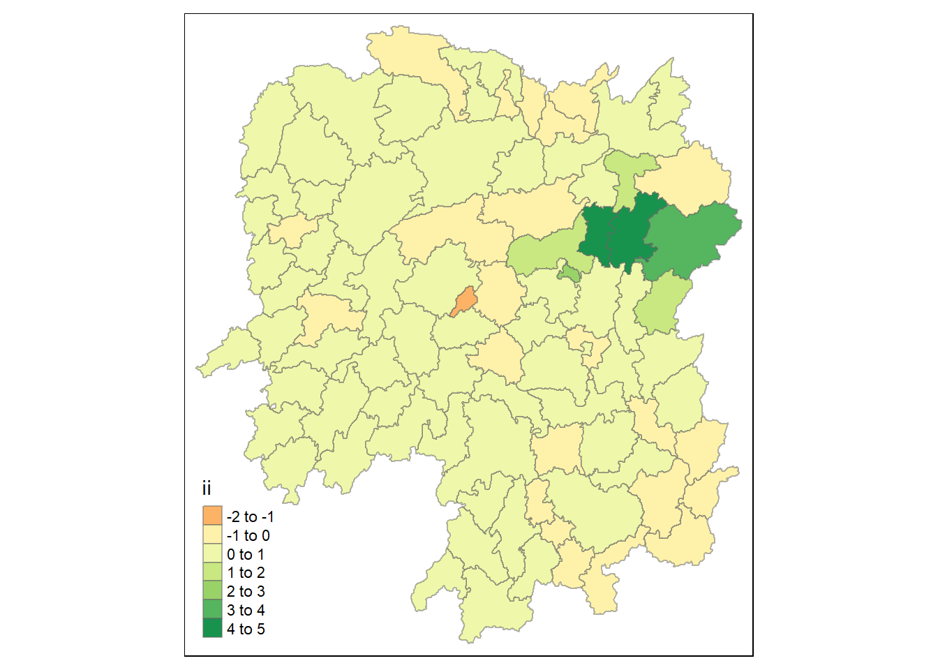

3.7.2 Computing p_ii

tmap_mode("plot")
tm_shape(lisa) +
  tm_fill("p_ii") +
  tm_borders(alpha = 0.5)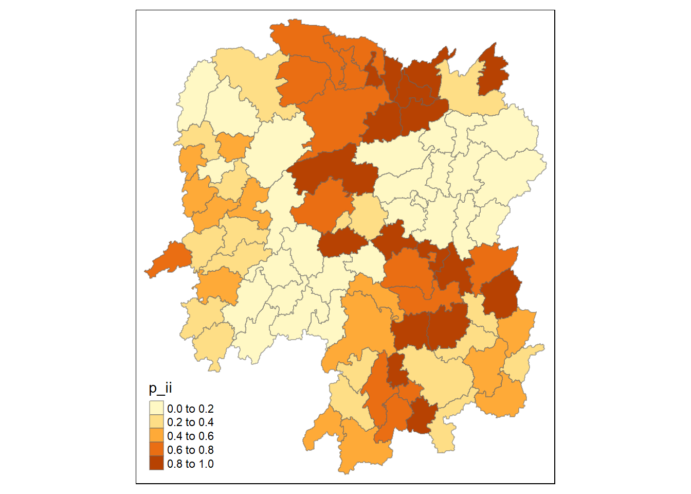

Ideally should use p_ii_sim variable of lisa so that results produced is stable.

3.7.3 Visualising the local Moran’s I Map

lisa_sig <- lisa %>%
  filter(p_ii < 0.05)
tmap_mode("plot")
tm_shape(lisa) +
  tm_polygons() +
  tm_borders(alpha = 0.5) +
tm_shape(lisa_sig) +
  tm_fill("mean") + 
  tm_borders(alpha = 0.4)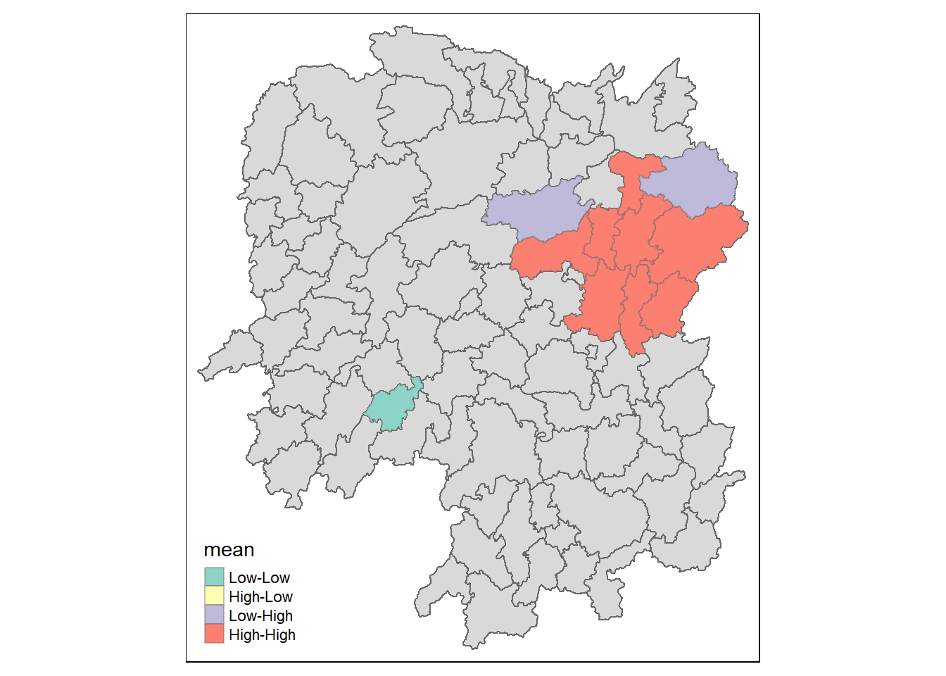

For take home exercise 2, add on to use insignificant on top of LL,HL,LH,HH, no need to use LISA but hot & cold spot areas

4. Hot Spot and Cold Spot Analysis

HCSA <- wm_q %>%
  mutate(local_GI = local_gstar_perm(
    GDPPC, nb, wt, nsim = 99),
    .before = 1) %>%
  unnest(local_GI)

HCSA

Simple feature collection with 88 features and 16 fields
Geometry type: POLYGON
Dimension:     XY
Bounding box:  xmin: 108.7831 ymin: 24.6342 xmax: 114.2544 ymax: 30.12812
Geodetic CRS:  WGS 84
# A tibble: 88 × 17
   gi_star   e_gi     var_gi p_value   p_sim p_fol…¹ skewn…² kurto…³ nb    wt   
     <dbl>  <dbl>      <dbl>   <dbl>   <dbl>   <dbl>   <dbl>   <dbl> <nb>  <lis>
 1  0.0416 0.0114 0.00000641  0.0493 9.61e-1    0.7     0.35   0.875 <int> <dbl>
 2 -0.333  0.0106 0.00000384 -0.0941 9.25e-1    1       0.5    0.661 <int> <dbl>
 3  0.281  0.0126 0.00000751 -0.151  8.80e-1    0.9     0.45   0.640 <int> <dbl>
 4  0.411  0.0118 0.00000922  0.264  7.92e-1    0.6     0.3    0.853 <int> <dbl>
 5  0.387  0.0115 0.00000956  0.339  7.34e-1    0.62    0.31   1.07  <int> <dbl>
 6 -0.368  0.0118 0.00000591 -0.583  5.60e-1    0.72    0.36   0.594 <int> <dbl>
 7  3.56   0.0151 0.00000731  2.61   9.01e-3    0.06    0.03   1.09  <int> <dbl>
 8  2.52   0.0136 0.00000614  1.49   1.35e-1    0.2     0.1    1.12  <int> <dbl>
 9  4.56   0.0144 0.00000584  3.53   4.17e-4    0.04    0.02   1.23  <int> <dbl>
10  1.16   0.0104 0.00000370  1.82   6.86e-2    0.12    0.06   0.416 <int> <dbl>
# … with 78 more rows, 7 more variables: NAME_2 <chr>, ID_3 <int>,
#   NAME_3 <chr>, ENGTYPE_3 <chr>, County <chr>, GDPPC <dbl>,
#   geometry <POLYGON [°]>, and abbreviated variable names ¹p_folded_sim,
#   ²skewness, ³kurtosis

4.1 Visualising Gi*

tmap_mode("view")
tm_shape(HCSA) +
  tm_fill("gi_star") +
  tm_borders(alpha = 0.5) +
  tm_view(set.zoom.limits = c(6,8))

4.2 Visualising the p value of HCSA

tmap_mode("plot")
tm_shape(HCSA) +
  tm_fill("p_sim") +
  tm_borders(alpha = 0.5)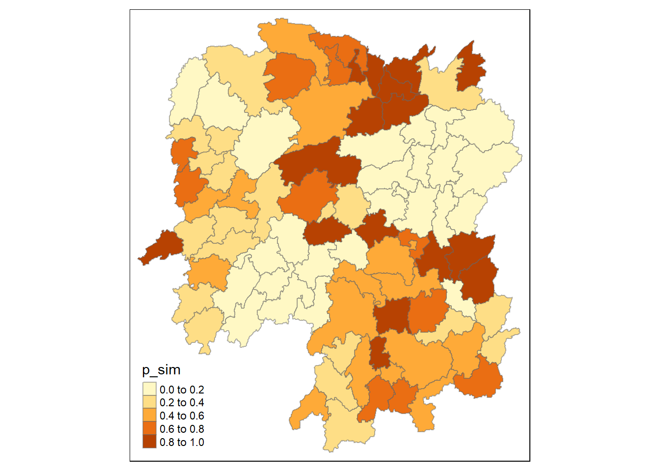

5. Mann-Kendall Test

5.1 Import files of Hunan GDPPC

GDPPC <- read_csv("Data/Aspatial/Hunan_GDPPC.csv")

5.1.1 Creating a time series cube

GDPPC_st <- spacetime(GDPPC, hunan,
                      .loc_col = "County",
                      .time_col = "Year")

To construct spacetime cube, we must obtain the location and time

GDPPC_nb <- GDPPC_st %>%
  activate("geometry") %>%
  mutate(
    nb = include_self(st_contiguity(geometry)),
    wt = st_weights(nb)
  ) %>%
  set_nbs("nb") %>%
  set_wts("wt")

5.2 Arrange to show significant hotspot and coldspot areas

5.3 Performing Emerging Hotspot Analysis

ehsa <- emerging_hotspot_analysis(
  x = GDPPC_st,
  .var = "GDPPC",
  k = 1,
  nsim = 99
)