pacman::p_load(dplyr, olsrr, corrplot, cowplot, sf, spdep, GWmodel, tmap, tidyverse, gtsummary, readr, ggpubr)In Class Exericse 8
13. Calibrating Hedonic Pricing Model for Private Highrise Property with GWR Method
13.1 Overview
Geographically weighted regression (GWR) is a spatial statistical technique that takes non-stationary variables into consideration (e.g., climate; demographic factors; physical environment characteristics) and models the local relationships between these independent variables and an outcome of interest (also known as dependent variable). In this hands-on exercise, you will learn how to build hedonic pricing models by using GWR methods. The dependent variable is the resale prices of condominium in 2015. The independent variables are divided into either structural and locational.
13.2 The Data
Two data sets will be used in this model building exercise, they are:
URA Master Plan subzone boundary in shapefile format (i.e. MP14_SUBZONE_WEB_PL)
condo_resale_2015 in csv format (i.e. condo_resale_2015.csv)
13.3 Getting Started
Before we get started, it is important for us to install the necessary R packages into R and launch these R packages into R environment.
The R packages needed for this exercise are as follows:
R package for building OLS and performing diagnostics tests
R package for calibrating geographical weighted family of models
R package for multivariate data visualisation and analysis
Spatial data handling
- sf
Attribute data handling
- tidyverse, especially readr, ggplot2 and dplyr
Choropleth mapping
- tmap
The code chunks below installs and launches these R packages into R environment.
13.4 A short note about the GWModel
GWmodel package provides a collection of localised spatial statistical methods, namely: GW summary statistics, GW principal components analysis, GW discriminant analysis and various forms of GW regression; some of which are provided in basic and robust (outlier resistant) forms. Commonly, outputs or parameters of the GWmodel are mapped to provide a useful exploratory tool, which can often precede (and direct) a more traditional or sophisticated statistical analysis.
13.5 Geospatial Data Wrangling
13.5.1 Importing Geospatial Data
The geospatial data used in this hands-on exercise is called MP14_SUBZONE_WEB_PL. It is in ESRI shapefile format. The shapefile consists of URA Master Plan 2014’s planning subzone boundaries. Polygon features are used to represent these geographic boundaries. The GIS data is in svy21 projected coordinates systems.
The code chunk below is used to import MP_SUBZONE_WEB_PL shapefile by using st_read() of sf packages.
mpsz = st_read(dsn = "data/geospatial", layer = "MP14_SUBZONE_WEB_PL")Reading layer `MP14_SUBZONE_WEB_PL' from data source
`C:\Users\kwekm\Desktop\SMU Year 3 Semester 2\IS415 Geospatial Analytics and Applications\KMRCrazyDuck\IS415-KMR\In-class_Ex\Data\Geospatial'
using driver `ESRI Shapefile'
Simple feature collection with 323 features and 15 fields
Geometry type: MULTIPOLYGON
Dimension: XY
Bounding box: xmin: 2667.538 ymin: 15748.72 xmax: 56396.44 ymax: 50256.33
Projected CRS: SVY21The report above shows that the R object used to contain the imported MP14_SUBZONE_WEB_PL shapefile is called mpsz and it is a simple feature object. The geometry type is multipolygon. it is also important to note that mpsz simple feature object does not have EPSG information.
13.5.2 Updating CRS information
The code chunk below updates the newly imported mpsz with the correct ESPG code (i.e. 3414)
mpsz_svy21 <- st_transform(mpsz, 3414)After transforming the projection metadata, you can varify the projection of the newly transformed mpsz_svy21 by using st_crs() of sf package.
The code chunk below will be used to varify the newly transformed mpsz_svy21.
st_crs(mpsz_svy21)Coordinate Reference System:
User input: EPSG:3414
wkt:
PROJCRS["SVY21 / Singapore TM",
BASEGEOGCRS["SVY21",
DATUM["SVY21",
ELLIPSOID["WGS 84",6378137,298.257223563,
LENGTHUNIT["metre",1]]],
PRIMEM["Greenwich",0,
ANGLEUNIT["degree",0.0174532925199433]],
ID["EPSG",4757]],
CONVERSION["Singapore Transverse Mercator",
METHOD["Transverse Mercator",
ID["EPSG",9807]],
PARAMETER["Latitude of natural origin",1.36666666666667,
ANGLEUNIT["degree",0.0174532925199433],
ID["EPSG",8801]],
PARAMETER["Longitude of natural origin",103.833333333333,
ANGLEUNIT["degree",0.0174532925199433],
ID["EPSG",8802]],
PARAMETER["Scale factor at natural origin",1,
SCALEUNIT["unity",1],
ID["EPSG",8805]],
PARAMETER["False easting",28001.642,
LENGTHUNIT["metre",1],
ID["EPSG",8806]],
PARAMETER["False northing",38744.572,
LENGTHUNIT["metre",1],
ID["EPSG",8807]]],
CS[Cartesian,2],
AXIS["northing (N)",north,
ORDER[1],
LENGTHUNIT["metre",1]],
AXIS["easting (E)",east,
ORDER[2],
LENGTHUNIT["metre",1]],
USAGE[
SCOPE["Cadastre, engineering survey, topographic mapping."],
AREA["Singapore - onshore and offshore."],
BBOX[1.13,103.59,1.47,104.07]],
ID["EPSG",3414]]Notice that the EPSG: is indicated as 3414 now.
Next, you will reveal the extent of mpsz_svy21 by using st_bbox() of sf package
13.6 Aspatial Data wrangling
13.6.1 Importing the Aspatial Data
The condo_resale_2015 is in csv file format. The codes chunk below uses read_csv() function of readr package to import condo_resale_2015 into R as a tibble data frame called condo_resale.
condo_resale = read_csv("data/aspatial/Condo_resale_2015.csv")After importing the data file into R, it is important for us to examine if the data file has been imported correctly.
The codes chunks below uses glimpse() to display the data structure of will do the job.
glimpse(condo_resale)Rows: 1,436
Columns: 23
$ LATITUDE <dbl> 1.287145, 1.328698, 1.313727, 1.308563, 1.321437,…
$ LONGITUDE <dbl> 103.7802, 103.8123, 103.7971, 103.8247, 103.9505,…
$ POSTCODE <dbl> 118635, 288420, 267833, 258380, 467169, 466472, 3…
$ SELLING_PRICE <dbl> 3000000, 3880000, 3325000, 4250000, 1400000, 1320…
$ AREA_SQM <dbl> 309, 290, 248, 127, 145, 139, 218, 141, 165, 168,…
$ AGE <dbl> 30, 32, 33, 7, 28, 22, 24, 24, 27, 31, 17, 22, 6,…
$ PROX_CBD <dbl> 7.941259, 6.609797, 6.898000, 4.038861, 11.783402…
$ PROX_CHILDCARE <dbl> 0.16597932, 0.28027246, 0.42922669, 0.39473543, 0…
$ PROX_ELDERLYCARE <dbl> 2.5198118, 1.9333338, 0.5021395, 1.9910316, 1.121…
$ PROX_URA_GROWTH_AREA <dbl> 6.618741, 7.505109, 6.463887, 4.906512, 6.410632,…
$ PROX_HAWKER_MARKET <dbl> 1.76542207, 0.54507614, 0.37789301, 1.68259969, 0…
$ PROX_KINDERGARTEN <dbl> 0.05835552, 0.61592412, 0.14120309, 0.38200076, 0…
$ PROX_MRT <dbl> 0.5607188, 0.6584461, 0.3053433, 0.6910183, 0.528…
$ PROX_PARK <dbl> 1.1710446, 0.1992269, 0.2779886, 0.9832843, 0.116…
$ PROX_PRIMARY_SCH <dbl> 1.6340256, 0.9747834, 1.4715016, 1.4546324, 0.709…
$ PROX_TOP_PRIMARY_SCH <dbl> 3.3273195, 0.9747834, 1.4715016, 2.3006394, 0.709…
$ PROX_SHOPPING_MALL <dbl> 2.2102717, 2.9374279, 1.2256850, 0.3525671, 1.307…
$ PROX_SUPERMARKET <dbl> 0.9103958, 0.5900617, 0.4135583, 0.4162219, 0.581…
$ PROX_BUS_STOP <dbl> 0.10336166, 0.28673408, 0.28504777, 0.29872340, 0…
$ NO_Of_UNITS <dbl> 18, 20, 27, 30, 30, 31, 32, 32, 32, 32, 34, 34, 3…
$ FAMILY_FRIENDLY <dbl> 0, 0, 0, 0, 0, 1, 1, 0, 1, 1, 0, 0, 0, 0, 0, 0, 0…
$ FREEHOLD <dbl> 1, 1, 1, 1, 1, 1, 1, 1, 1, 0, 1, 1, 1, 1, 1, 1, 1…
$ LEASEHOLD_99YR <dbl> 0, 0, 0, 0, 0, 0, 0, 0, 0, 0, 0, 0, 0, 0, 0, 0, 0…head(condo_resale$LONGITUDE) #see the data in XCOORD column[1] 103.7802 103.8123 103.7971 103.8247 103.9505 103.9386head(condo_resale$LATITUDE) #see the data in YCOORD column[1] 1.287145 1.328698 1.313727 1.308563 1.321437 1.314198Next, summary() of base R is used to display the summary statistics of condo_resale tibble data frame.
summary(condo_resale) LATITUDE LONGITUDE POSTCODE SELLING_PRICE
Min. :1.240 Min. :103.7 Min. : 18965 Min. : 540000
1st Qu.:1.309 1st Qu.:103.8 1st Qu.:259849 1st Qu.: 1100000
Median :1.328 Median :103.8 Median :469298 Median : 1383222
Mean :1.334 Mean :103.8 Mean :440439 Mean : 1751211
3rd Qu.:1.357 3rd Qu.:103.9 3rd Qu.:589486 3rd Qu.: 1950000
Max. :1.454 Max. :104.0 Max. :828833 Max. :18000000
AREA_SQM AGE PROX_CBD PROX_CHILDCARE
Min. : 34.0 Min. : 0.00 Min. : 0.3869 Min. :0.004927
1st Qu.:103.0 1st Qu.: 5.00 1st Qu.: 5.5574 1st Qu.:0.174481
Median :121.0 Median :11.00 Median : 9.3567 Median :0.258135
Mean :136.5 Mean :12.14 Mean : 9.3254 Mean :0.326313
3rd Qu.:156.0 3rd Qu.:18.00 3rd Qu.:12.6661 3rd Qu.:0.368293
Max. :619.0 Max. :37.00 Max. :19.1804 Max. :3.465726
PROX_ELDERLYCARE PROX_URA_GROWTH_AREA PROX_HAWKER_MARKET PROX_KINDERGARTEN
Min. :0.05451 Min. :0.2145 Min. :0.05182 Min. :0.004927
1st Qu.:0.61254 1st Qu.:3.1643 1st Qu.:0.55245 1st Qu.:0.276345
Median :0.94179 Median :4.6186 Median :0.90842 Median :0.413385
Mean :1.05351 Mean :4.5981 Mean :1.27987 Mean :0.458903
3rd Qu.:1.35122 3rd Qu.:5.7550 3rd Qu.:1.68578 3rd Qu.:0.578474
Max. :3.94916 Max. :9.1554 Max. :5.37435 Max. :2.229045
PROX_MRT PROX_PARK PROX_PRIMARY_SCH PROX_TOP_PRIMARY_SCH
Min. :0.05278 Min. :0.02906 Min. :0.07711 Min. :0.07711
1st Qu.:0.34646 1st Qu.:0.26211 1st Qu.:0.44024 1st Qu.:1.34451
Median :0.57430 Median :0.39926 Median :0.63505 Median :1.88213
Mean :0.67316 Mean :0.49802 Mean :0.75471 Mean :2.27347
3rd Qu.:0.84844 3rd Qu.:0.65592 3rd Qu.:0.95104 3rd Qu.:2.90954
Max. :3.48037 Max. :2.16105 Max. :3.92899 Max. :6.74819
PROX_SHOPPING_MALL PROX_SUPERMARKET PROX_BUS_STOP NO_Of_UNITS
Min. :0.0000 Min. :0.0000 Min. :0.001595 Min. : 18.0
1st Qu.:0.5258 1st Qu.:0.3695 1st Qu.:0.098356 1st Qu.: 188.8
Median :0.9357 Median :0.5687 Median :0.151710 Median : 360.0
Mean :1.0455 Mean :0.6141 Mean :0.193974 Mean : 409.2
3rd Qu.:1.3994 3rd Qu.:0.7862 3rd Qu.:0.220466 3rd Qu.: 590.0
Max. :3.4774 Max. :2.2441 Max. :2.476639 Max. :1703.0
FAMILY_FRIENDLY FREEHOLD LEASEHOLD_99YR
Min. :0.0000 Min. :0.0000 Min. :0.0000
1st Qu.:0.0000 1st Qu.:0.0000 1st Qu.:0.0000
Median :0.0000 Median :0.0000 Median :0.0000
Mean :0.4868 Mean :0.4227 Mean :0.4882
3rd Qu.:1.0000 3rd Qu.:1.0000 3rd Qu.:1.0000
Max. :1.0000 Max. :1.0000 Max. :1.0000 13.6.2 Converting aspatial data frame into a sf object
Currently, the condo_resale tibble data frame is Aspatial. We will convert it to a sf object. The code chunk below converts condo_resale data frame into a simple feature data frame by using st_as_sf() of sf packages.
condo_resale.sf <- st_as_sf(condo_resale,
                            coords = c("LONGITUDE", "LATITUDE"),
                            crs=4326) %>%
  st_transform(crs=3414)
Notice that st_transform() of sf package is used to convert the coordinates from wgs84 (i.e. crs:4326) to svy21 (i.e. crs=3414).
Next, head() is used to list the content of condo_resale.sf object.
head(condo_resale.sf)Simple feature collection with 6 features and 21 fields
Geometry type: POINT
Dimension: XY
Bounding box: xmin: 22085.12 ymin: 29951.54 xmax: 41042.56 ymax: 34546.2
Projected CRS: SVY21 / Singapore TM
# A tibble: 6 × 22
POSTCODE SELLI…¹ AREA_…² AGE PROX_…³ PROX_…⁴ PROX_…⁵ PROX_…⁶ PROX_…⁷ PROX_…⁸
<dbl> <dbl> <dbl> <dbl> <dbl> <dbl> <dbl> <dbl> <dbl> <dbl>
1 118635 3000000 309 30 7.94 0.166 2.52 6.62 1.77 0.0584
2 288420 3880000 290 32 6.61 0.280 1.93 7.51 0.545 0.616
3 267833 3325000 248 33 6.90 0.429 0.502 6.46 0.378 0.141
4 258380 4250000 127 7 4.04 0.395 1.99 4.91 1.68 0.382
5 467169 1400000 145 28 11.8 0.119 1.12 6.41 0.565 0.461
6 466472 1320000 139 22 10.3 0.125 0.789 5.09 0.781 0.0994
# … with 12 more variables: PROX_MRT <dbl>, PROX_PARK <dbl>,
# PROX_PRIMARY_SCH <dbl>, PROX_TOP_PRIMARY_SCH <dbl>,
# PROX_SHOPPING_MALL <dbl>, PROX_SUPERMARKET <dbl>, PROX_BUS_STOP <dbl>,
# NO_Of_UNITS <dbl>, FAMILY_FRIENDLY <dbl>, FREEHOLD <dbl>,
# LEASEHOLD_99YR <dbl>, geometry <POINT [m]>, and abbreviated variable names
# ¹SELLING_PRICE, ²AREA_SQM, ³PROX_CBD, ⁴PROX_CHILDCARE, ⁵PROX_ELDERLYCARE,
# ⁶PROX_URA_GROWTH_AREA, ⁷PROX_HAWKER_MARKET, ⁸PROX_KINDERGARTENNotice that the output is in point feature data frame.
13.7 Exploratory Data Analysis (EDA)
In the section, you will learn how to use statistical graphics functions of ggplot2 package to perform EDA.
13.7.1 EDA using statistical graphics
We can plot the distribution of SELLING_PRICE by using appropriate Exploratory Data Analysis (EDA) as shown in the code chunk below.
ggplot(data=condo_resale.sf, aes(x=`SELLING_PRICE`)) +
  geom_histogram(bins=20, color="black", fill="light blue")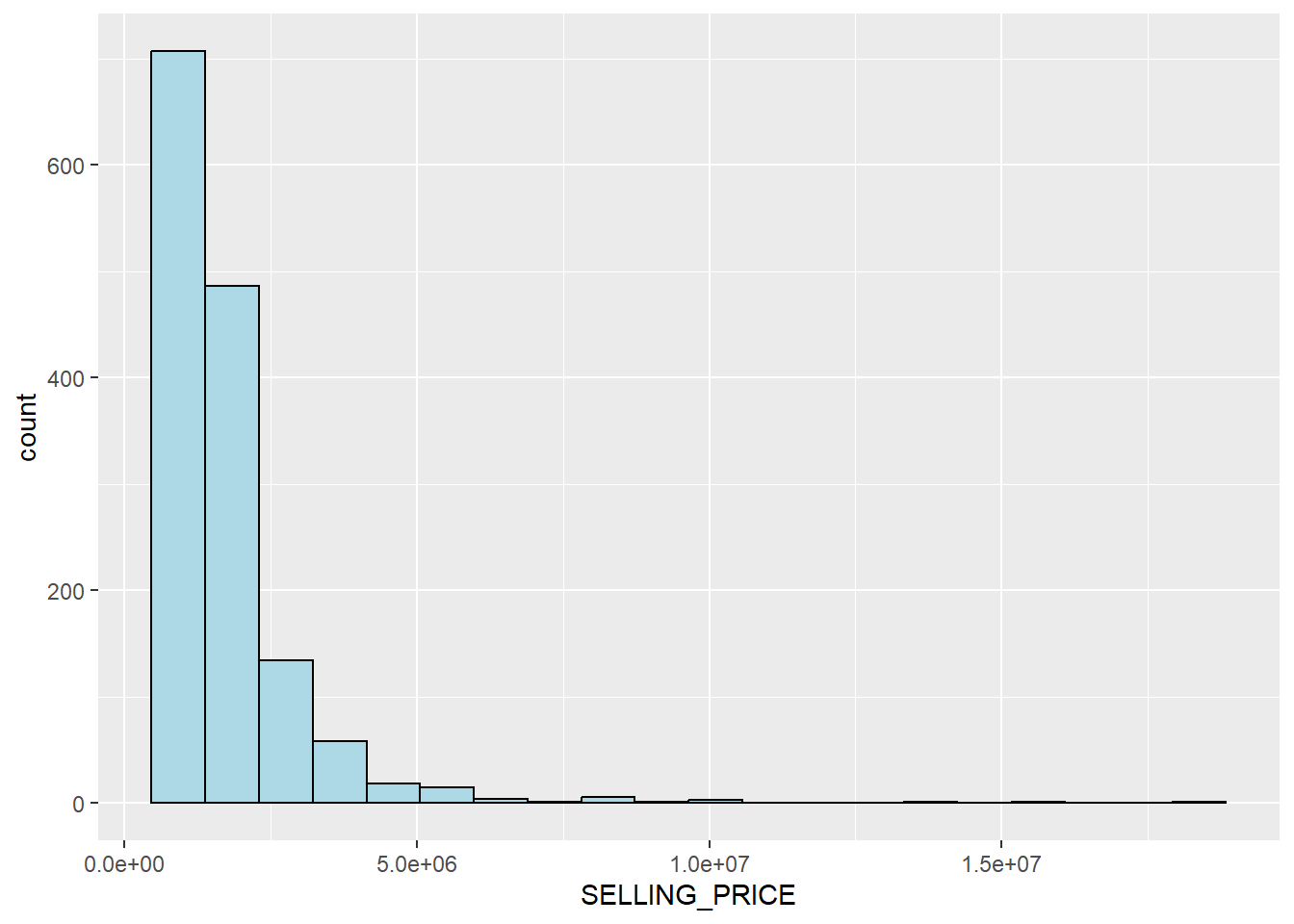
The figure above reveals a right skewed distribution. This means that more condominium units were transacted at relative lower prices.
Statistically, the skewed dsitribution can be normalised by using log transformation. The code chunk below is used to derive a new variable called LOG_SELLING_PRICE by using a log transformation on the variable SELLING_PRICE. It is performed using mutate() of dplyr package.
condo_resale.sf <- condo_resale.sf %>%
  mutate(`LOG_SELLING_PRICE` = log(SELLING_PRICE))
Now, you can plot the LOG_SELLING_PRICE using the code chunk below.
ggplot(data=condo_resale.sf, aes(x=`LOG_SELLING_PRICE`)) +
  geom_histogram(bins=20, color="black", fill="light blue")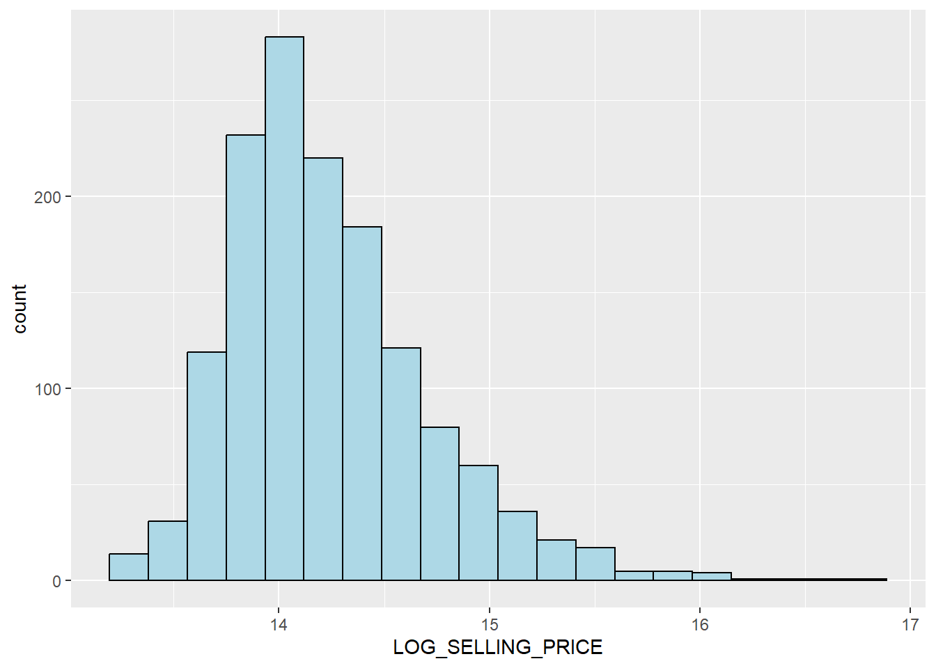
Notice that the distribution is relatively less skewed after the transformation.
13.7.2 Multiple Histogram Plots distribution of variables
In this section, you will learn how to draw a small multiple histograms (also known as trellis plot) by using ggarrange() of ggpubr package.
The code chunk below is used to create 12 histograms. Then, ggarrange() is used to organised these histogram into a 3 columns by 4 rows small multiple plot.
AREA_SQM <- ggplot(data=condo_resale.sf, aes(x= `AREA_SQM`)) +
  geom_histogram(bins=20, color="black", fill="light blue")

AGE <- ggplot(data=condo_resale.sf, aes(x= `AGE`)) +
  geom_histogram(bins=20, color="black", fill="light blue")

PROX_CBD <- ggplot(data=condo_resale.sf, aes(x= `PROX_CBD`)) +
  geom_histogram(bins=20, color="black", fill="light blue")

PROX_CHILDCARE <- ggplot(data=condo_resale.sf, aes(x= `PROX_CHILDCARE`)) +
  geom_histogram(bins=20, color="black", fill="light blue")

PROX_ELDERLYCARE <- ggplot(data=condo_resale.sf, aes(x= `PROX_ELDERLYCARE`)) +
  geom_histogram(bins=20, color="black", fill="light blue")

PROX_URA_GROWTH_AREA <- ggplot(data=condo_resale.sf,
                               aes(x= `PROX_URA_GROWTH_AREA`)) +
  geom_histogram(bins=20, color="black", fill="light blue")

PROX_HAWKER_MARKET <- ggplot(data=condo_resale.sf, aes(x= `PROX_HAWKER_MARKET`)) +
  geom_histogram(bins=20, color="black", fill="light blue")

PROX_KINDERGARTEN <- ggplot(data=condo_resale.sf, aes(x= `PROX_KINDERGARTEN`)) +
  geom_histogram(bins=20, color="black", fill="light blue")

PROX_MRT <- ggplot(data=condo_resale.sf, aes(x= `PROX_MRT`)) +
  geom_histogram(bins=20, color="black", fill="light blue")

PROX_PARK <- ggplot(data=condo_resale.sf, aes(x= `PROX_PARK`)) +
  geom_histogram(bins=20, color="black", fill="light blue")

PROX_PRIMARY_SCH <- ggplot(data=condo_resale.sf, aes(x= `PROX_PRIMARY_SCH`)) +
  geom_histogram(bins=20, color="black", fill="light blue")

PROX_TOP_PRIMARY_SCH <- ggplot(data=condo_resale.sf,
                               aes(x= `PROX_TOP_PRIMARY_SCH`)) +
  geom_histogram(bins=20, color="black", fill="light blue")

ggarrange(AREA_SQM, AGE, PROX_CBD, PROX_CHILDCARE, PROX_ELDERLYCARE,
          PROX_URA_GROWTH_AREA, PROX_HAWKER_MARKET, PROX_KINDERGARTEN, PROX_MRT,
          PROX_PARK, PROX_PRIMARY_SCH, PROX_TOP_PRIMARY_SCH,
          ncol = 3, nrow = 4)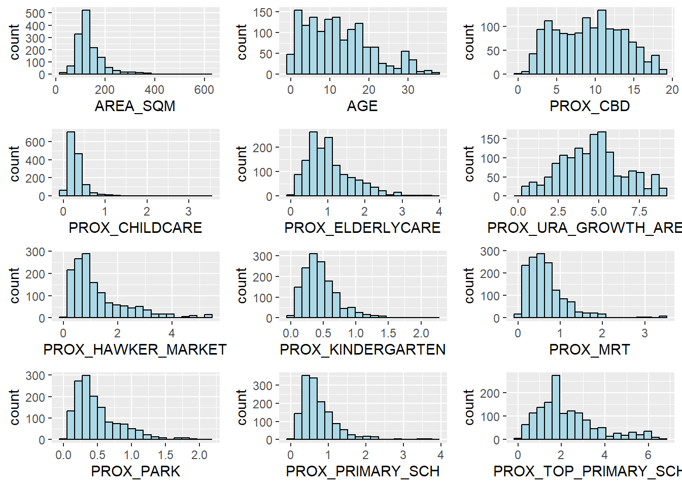
13.7.3 Drawing Statistical Point Map
Lastly, we want to reveal the geospatial distribution condominium resale prices in Singapore. The map will be prepared by using tmap package.
First, we will turn on the interactive mode of tmap by using the code chunk below
tmap_mode("view")Next, the code chunks below is used to create an interactive point symbol map.
sf_use_s2(FALSE)

tm_shape(mpsz_svy21)+
  tm_polygons() +
tm_shape(condo_resale.sf) +
  tm_dots(col = "SELLING_PRICE",
          alpha = 0.6,
          style="quantile") +
  tm_view(set.zoom.limits = c(11,14))
Notice that tm_dots() is used instead of tm_bubbles().
set.zoom.limits argument of tm_view() sets the minimum and maximum zoom level to 11 and 14 respectively.
Before moving on to the next section, the code below will be used to turn R display into plot mode.
tmap_mode("plot")13.8 Hedonic Pricing Modelling in R
In this section, you will learn how to building hedonic pricing models for condominium resale units using lm() of R base.
13.8.1 Simple Linear Regression Method
First, we will build a simple linear regression model by using SELLING_PRICE as the dependent variable and AREA_SQM as the independent variable.
condo.slr <- lm(formula=SELLING_PRICE ~ AREA_SQM, data = condo_resale.sf)lm() returns an object of class “lm” or for multiple responses of class c(“mlm”, “lm”).
The functions summary() and anova() can be used to obtain and print a summary and analysis of variance table of the results. The generic accessor functions coefficients, effects, fitted.values and residuals extract various useful features of the value returned by lm.
summary(condo.slr)
Call:
lm(formula = SELLING_PRICE ~ AREA_SQM, data = condo_resale.sf)

Residuals:
     Min       1Q   Median       3Q      Max
-3695815  -391764   -87517   258900 13503875

Coefficients:
             Estimate Std. Error t value Pr(>|t|)
(Intercept) -258121.1    63517.2  -4.064 5.09e-05 ***
AREA_SQM      14719.0      428.1  34.381  < 2e-16 ***
---
Signif. codes:  0 '***' 0.001 '**' 0.01 '*' 0.05 '.' 0.1 ' ' 1

Residual standard error: 942700 on 1434 degrees of freedom
Multiple R-squared:  0.4518,    Adjusted R-squared:  0.4515
F-statistic:  1182 on 1 and 1434 DF,  p-value: < 2.2e-16
Call: lm(formula = SELLING_PRICE ~ AREA_SQM, data = condo_resale.sf)
Residuals: Min 1Q Median 3Q Max -3695815 -391764 -87517 258900 13503875
Coefficients: Estimate Std. Error t value Pr(>|t|)
(Intercept) -258121.1 63517.2 -4.064 5.09e-05 AREA_SQM 14719.0 428.1 34.381 < 2e-16
Signif. codes: 0 ‘’ 0.001 ’’ 0.01 ’’ 0.05 ‘.’ 0.1 ’ ’ 1
Residual standard error: 942700 on 1434 degrees of freedom Multiple R-squared: 0.4518, Adjusted R-squared: 0.4515 F-statistic: 1182 on 1 and 1434 DF, p-value: < 2.2e-16 The output report reveals that the SELLING_PRICE can be explained by using the formula:
*y = -258121.1 + 14719x1*The R-squared of 0.4518 reveals that the simple regression model built is able to explain about 45% of the resale prices.
Since p-value is much smaller than 0.0001, we will reject the null hypothesis that mean is a good estimator of SELLING_PRICE. This will allow us to infer that simple linear regression model above is a good estimator of SELLING_PRICE.
The Coefficients: section of the report reveals that the p-values of both the estimates of the Intercept and ARA_SQM are smaller than 0.001. In view of this, the null hypothesis of the B0 and B1 are equal to 0 will be rejected. As a results, we will be able to infer that the B0 and B1 are good parameter estimates.
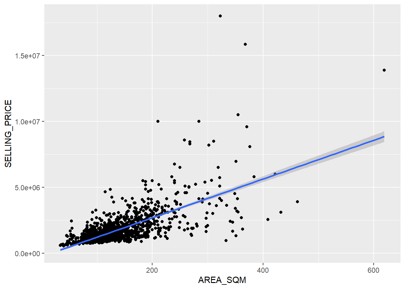
To visualise the best fit curve on a scatterplot, we can incorporate lm() as a method function in ggplot’s geometry as shown in the code chunk below.
ggplot(data=condo_resale.sf,
       aes(x=`AREA_SQM`, y=`SELLING_PRICE`)) +
  geom_point() +
  geom_smooth(method = lm)